7.1.3 Off scanning line

Sweep line algorithm

Set up a horizontal scan line that sweeps across each vertex from top to bottom. For each point, proceed according to its type. For start points, end points and ordinary points, the boundary information of small polygons is maintained. For split points, inner diagonals are connected and the polygon is split.
The same goes for merging points, just doing it again from the bottom up.

Required data structure: Since we need to find and maintain the current boundary of each small polygon, a binary search tree is used.

Specifically: for each point scanned from top to bottom for the first time, what we have to do is:

Starting point: Indicates that a new small polygon is started, and its left and right boundaries are added to the tree.
End point: It means that a small polygon ends. Find the left and right boundaries of the end point and delete it from the tree.
Split point: Find the left and right boundaries of the polygon where this point is located and the nearest point above the point from the tree, connect the inner diagonal, add the information of the two new polygons, and delete the old polygon.
Merge points: This time we do not connect the diagonals (only in the second bottom-to-top scan), we only need to merge the boundary information of two small polygons into a polygon and add the tree.
Ordinary points: Maintain the boundary information of the current polygon.

This algorithm is relatively complex and contains a large amount of information. It can be combined with the scanning process in the figure below to manually simulate it to help understand it.

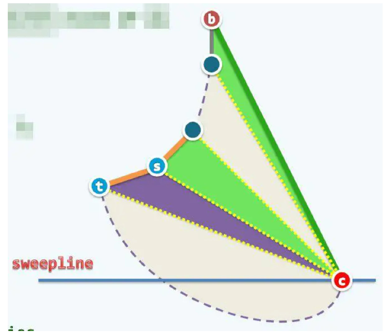
Figure 1 Scan line algorithm

time complexity

sort $O(nlogn)$ , during the scanning process, it is necessary to find and maintain a binary balanced tree for each point, which costs every time $O(logn)$ , a total of $n$ point. So the total complexity $O(nlogn)$ 。

Triangulating Monotone Polygons

Since monotonic polygons have good properties, we can start from the greedy idea and gradually scan down along the left and right boundaries of the polygon, operating when we encounter a vertex.

monotonic stack

You can consider when a triangle can be divided when a point is scanned, and when it cannot. For example:

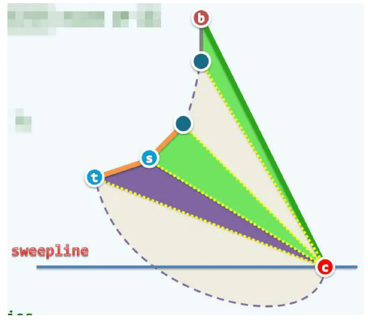
Figure 2 Triangulation polygon

Case 1

When a point is scanned and is on the opposite side to the previous point, it can be connected to the previous point in sequence for triangulation until all the points on the opposite side are used up.

Case 2

When the point is scanned, it is on the same side as the previous two points, and the internal angle formed is , it can be connected with the first two points to split a triangle, and the point after splitting will be invalid. If the internal angle formed with the first two points is still , continue splitting.

Case 3

When the point is scanned, it cannot be divided into a triangle only when it is on the same side as the previous two points and the interior angle formed is .

If you have learned $Graham$ If you use the scanning method to find the convex hull, you will definitely find that they are very similar. So we use a monotonic stack to save the information of the previous point. The elements in the monotonic stack satisfy:

Increasing height: Because we scan from top to bottom, the top element of the stack must be the lowest.
On the same side: If there are elements on different sides, you can continue to divide them upward until the remaining elements are all on the same side.
The interior angle between three consecutive elements in the stack $> i$ (monotonicity).

Scan line algorithm

Similar to the previous scan line algorithm, a horizontal scan line is set up from top to bottom. The highest point is added to the stack at the beginning, and then scans downward. Each point is operated according to the above classification.

Since this algorithm is relatively simple, each step is not described in detail here, only the code is given.

code

The following code is for reference only and to help understand the algorithm. In fact, many $corner$ $case$ For example, if three points are collinear or if two points have the same ordinate, they are not considered, so there is almost no robustness. This code is only able to give the correct diagonal given the very normal case of a monotonic polygon.

Input: $n$ points, polygon coordinates given counterclockwise: $p_0:(x_0,y_0),p_1:(x_1,y_1),...... ,p_{n-1}:(x_{n-1}, y_{n-1})$ 。
Output: Numbers of two points connected by several diagonal lines $a,b$ , represents the point $p_a$ and $p_b$ connected.

#include <bits/stdc++.h>
using namespace std;
typedef double db;
const db eps = 1e-6;
int sign(db k)
{ if (k > eps) return 1; else if (k < -eps) return -1; return 0;
}
int cmp(db k1, db k2) { return sign(k1 - k2); }
struct point
{ db x, y; point operator+(const point &k1) const { return (point){k1.x + x, k1.y + y}; } point operator-(const point &k1) const { return (point){x - k1.x, y - k1.y}; } point operator*(db k1) const { return (point){x * k1, y * k1}; } point operator/(db k1) const { return (point){x / k1, y / k1}; } int operator==(const point &k1) const { return cmp(x, k1.x) == 0 && cmp(y, k1.y) == 0; } bool operator<(const point k1) const { int a = cmp(y, k1.y); if (a == -1) return 0; else if (a == 1) return 1; else return cmp(x, k1.x) == 1; }
};
db cross(point k1, point k2) { return k1.x * k2.y - k1.y * k2.x; }
db dot(point k1, point k2) { return k1.x * k2.x + k1.y * k2.y; } //-------------------------------------------------------- const int maxn = 1e5 + 10; int side[maxn]; vector<pair<int, int>> TriangulateMonotonePolygon(vector<pair<point, int>> v)
{ if (v.size() <= 3) return {}; vector<pair<int, int>> ans; int n = v.size(); auto vv = v; sort(vv.begin(), vv.end()); for (int i = (vv[0].second + 1) % n; i < vv[n - 1].second; i = (i + 1) % n) side[i] = 0; //* left: 0 right: 1 for (int i = (vv[n - 1].second + 1) % n; i < vv[0].second; i = (i + 1) % n) side[i] = 1; sort(v.begin(), v.end()); stack<pair<point, int>> st; st.push(v[0]); st.push(v[1]); for (int i = 2, sd = side[v[i].second]; i < n - 1; i++) { if (side[v[i].second] == side[st.top().second]) //same side { if (st.size() < 2) { st.push(v[i]); continue; } while (st.size() >= 2) { auto top = st.top(); st.pop(); auto top2 = st.top(); if (sd == 0 && sign(cross(top.first - top2.first, v[i].first - top.first)) == -1 || (sd == 1 && sign(cross(top.first - top2.first, v[i].first - top.first)) == 1)) { st.push(top); break; } ans.emplace_back(v[i].second, top2.second); } st.push(v[i]); } else { auto top = st.top(); while (st.size() > 1) { ans.emplace_back(v[i].second, st.top().second); st.pop(); } st.pop(); st.push(top); st.push(v[i]); } } int cnt = st.size(), now = st.size(); while (!st.empty()) { if (now == cnt || now == 1) { st.pop(); continue; } ans.emplace_back(v[n - 1].second, st.top().second); st.pop(); } return ans;
} vector<pair<point, int>> input; int main()
{ int n; cin >> n; input.resize(n); for (int i = 0; i < n; i++) cin >> input[i].first.x >> input[i].first.y, input[i].second = i; auto ans = TriangulateMonotonePolygon(input); cout << "diagonal id:" << endl; for (auto x : ans) cout << x.first << " " << x.second << endl;
}

time complexity

sort $O(nlogn)$ . Since each point in the monotonic stack will only be pushed into and popped out of the stack once, it will be evenly distributed. $O(1)$ , there is $n$ point, so $O(n)$ . total complexity $O(nlogn)$ 。
In fact, if the given monotonic polygons have been sorted and the left and right boundaries have been marked, the complexity of the sorting can be removed, and the total complexity of this part becomes $O(n)$ . This step can be done during monotonic polygon decomposition.

7.1.3 Off scanning line

# Sweep line algorithm

Figure 1 Scan line algorithm

# time complexity

# Triangulating Monotone Polygons

# monotonic stack

Figure 2 Triangulation polygon

# Scan line algorithm

# code

# time complexity

Sweep line algorithm

time complexity

Triangulating Monotone Polygons

monotonic stack

Scan line algorithm

code

time complexity